
Useful Links - Calculate IMU and Camera Timestamp Offset
")


Determining the Orientation
The IMU orientation plays a relevant role since there can be different physical configurations or hardware mountings. For instance, the camera can be straight, but the IMU can be upside down. It implies that the measurements change signs or swaps amongst them.
To fix possible axes exchange, it is possible to utilise two techniques:
1) Using the datasheet to determine the IMU position: This one allows you to know the axis from the IMU sensor.
2) Using the video movements until reaching the correct orientation: This option is more empirical, but provides an interactive way to get the correct axis.
Understanding the Axes and Mapping System
In the context of imaging, we assume that the image is represented in a 2D plane with X and Y axes, representing the horizontal and vertical positions, respectively. However, the actual camera movement can also include depth changes, represented in the Z axis, as follows:

Given how the image is represented digitally (pixel coordinates), the Y is a negative axis in this context.
On the other hand, the IMU can be placed given a rotation: flipped horizontally, vertically, or rotated. In this case, we are going to explain how to determine the orientation given a use case.

In the use case presented above, the camera has an IMU placed vertically, with the top looking at the camera's left side. Moreover, the IMU coordinates are presented in terms of the chip's first pin (reference pin).
The RidgeRun Video Stabilization library allows the user to choose the orientation of the axes. In this case, we represent the mapping as follows:

Given an orientation array of three fields, it is possible to assign the mapping from the sensor reference system to the image reference system. In this case, the order of the array provides the axes of the image reference system in the X, Y, Z order. The content of the array provides the axes in the sensor reference system. In the example, the mapping is the following:
Image     Sensor
  X   ->    z
  Y   ->    Y
  Z   ->    x
Please, pay attention to the camera orientation, which is affected by the view and orientation. In the end, the final image view is taken into account and not the lens orientation, given that optical reflections can happen in the process.
Using the Datasheet
IMU datasheets often offer information about the orientation of the movements with respect to the chip orientation.

The image above illustrates a redrawn diagram extracted from the BMI160 documentation next to the camera and its axes. The idea is to place the IMU in the camera in a certain orientation and then match the axes mapping with the orientation array. To illustrate this, please, refer to the following use case, where the sensor is vertically placed:

In this particular case, the sensor mapping process involves rotating the sensor until the axes match. In this case, the Z axis requires inversion, which implies that the orientation array should be defined as 'X', 'Y', and 'z'.
Using the Live Video
When using the live video, the idea is to iterate the orientation array by swapping those axes that provoke movements in a opposite direction from the supposed ones. The supposed video movement is as follows:

The camera's movements must counter the movement of the image window. In the image from above, when the camera is moved up, the image moves down. When the camera is moved to the right, the image moves to the left.
In case of a mismatch, it is critical to identify how it is moved to match the video. In this case, if the camera moves left and the image goes up, it is possible that the X and Y are swapped and one of them is inverted.
This is an empirical and iterative method through trial and error.
For easiness, we propose a tool to assist in the calibration of the IMU.
Remote Web Tool
The web tool available to run the IMU calibration provides and great way to get the right axis mapping and camera timestamp offset, it runs a UI in a browser. You'll need to make sure you have all requirements mentioned in the Calibration Process/Installing section.
The web tool consist of the following main parts:
- Device connection and login.
- You'll need to ensure the target device is reachable through ssh from the host device.
- Video capture and IMU data capture.
- The IMU and video capture parameters shows the required parameters, note that you need a camera
calibration.ymlfile ready (see Camera Calibration).
- The IMU and video capture parameters shows the required parameters, note that you need a camera
- Offset and IMU orientation calculation.
- Results display.
- All results are saved to the selected output directory.
The following video exemplifies the usage of this web tool for IMU Calibration. Also see the Recommended calibration techniques to ensure a good calibration setup and scene.
Note: The process can also be done from the terminal, directly on the target device. See the section below Calibrating using the local tool for further details.
Alternative 1: Calibrating using the local tool
Calculate IMU and Camera Timestamp Offset
This guide explains how to calculate the timestamp offset between IMU and camera streams using data captured with python tool.
The workflow is:
- Build all required components.
- Prepare the Python tool
- Capture data and offset calculation.
- Capture data and offset calculation
- Capture data and offset separate calculation
- Understanding the Results
1) Build dependencies and project
Make sure the project is built and installed as described in Building the Library section.
Also, make sure that your IMU driver is already supported on your device.
If you are using a Jetson platform with the ICM42688 IMU, follow the ICM42688 Setup. If you have the BMI160 IMU instead, follow the BMI160 Setup. The following example uses this sensor. This can be set through the Python tool options (--imu-sensor and --imu-sensor-device).
For camera source nvarguscamerasrc and rrv4l2src are supported by default with the --format option, but custom ones can be added by rewriting the capture pipeline with --pipeline (further details below).
2) Prepare the Python tool
First install uv:
sudo apt install curl
curl -LsSf https://astral.sh/uv/install.sh | sh
Inside the stabilizer project, navigate to the tools directory and install dependencies:
cd tools/calibration-tool/imu
uv sync
To see available options
uv run -m calibrator --help
uv run -m calibrator capture --help
uv run -m calibrator offset --help
uv run -m calibrator live-offset --help
captureoption only does capture of data as mentioned before.offsetdoes only calculation of offset and axis mapping.live-offsetdoes both capture and offset calculation.
3) Capture data and offset calculation
As mentioned before, you can run either each step separately or together with the live-offset option.
If you are going to use the calibration tool, it is strongly recommended to follow the calibration techniques described below.
Recommended calibration techniques
The accuracy of the timestamp offset and axis alignment estimation strongly depends on the quality and diversity of the captured motion. The following recommendations help produce richer motion data and improve the correlation between IMU measurements and optical-flow-derived angular velocities.
- IMU Positioning
- The IMU should ideally be placed as close as possible to the optical center of the camera, which is approximately the center of the image sensor along the optical axis.
- By keeping the IMU near the camera’s optical center, both sensors effectively share the same rotational reference point, simplifying the motion model and improving the stability and accuracy of the calibration.
- Here's an example of the positioning:
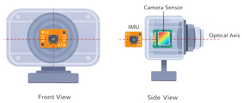
IMU position example

- Camera Motion
-
- Perform multiple rotations per axis
- Execute several rotations for each axis instead of only a few movements. For example:
- X axis: ~6 rotations
- Y axis: ~8 rotations
- Z axis: ~10 rotations
- This improves motion coverage and provides more samples for the cross-correlation process.
- Rotate in both directions
- Perform rotations in both directions relative to the initial orientation as in this example:
- Start from a neutral position.
- Rotate to one side up to the desired angle.
- Return to the neutral position.
- Rotate to the opposite side with approximately the same magnitude.
- Avoid performing movements only in one direction, as symmetric rotations improve correlation between IMU and optical flow signals.
- Pause briefly between movements
- When changing rotation direction, return to the neutral position and pause briefly before the next movement. This pause helps the optical flow (OF) algorithm better distinguish individual motion segments and improves the estimation of angular velocities.
The following images show the proper motion mentioned before:
-
 Axis X rotation
 -
 Axis Y rotation
 -
 Axis Z rotation


- Ensure proper scene conditions
-
- Use a well-illuminated environment.
- Ensure the scene contains sufficient visual objects or features.
- If possible, keep a distinct object near the center of the frame to provide stable tracking references.
- Avoid flat or featureless scenes, as they reduce the effectiveness of optical flow estimation.
Following these recommendations typically results in stronger correlations between IMU and optical flow signals, leading to more reliable timestamp offset and axis mapping estimation.
NOTE: For a better calibration consider to set a high --framerate and at least 5x that framerate for --imu-frequency. |
3a) Capture data and offset calculation
For this case we will run it together, since live-offset option also comes with instructions for the camera movements. Make sure you set the path to the calibration.yml file appropriately with --calibration option.
Run the calibrator capture you can use --write-csv to save the csv files to analyze later, but all calculation will be done in place, here's an example using an IMX477 camera with the icm42688 IMU:
uv run -m calibrator live-offset --calibration calibration.yml --duration-s 25 --format raw --video-out capture.mp4 --write-csv --plot --imu-sensor icm42600 --imu-sensor-device icm42688
Instructions will be printed, feel free to read it once and re run the calibration:
Capture instructions:
- Total duration: 25.00s
- Stage length: 4.80s (5 stages)
- Ensure good lighting and clear visual texture.
- Avoid camera-mounted objects in view (they stay fixed in the frame when the camera moves and degrade optical flow).
- Keep the motion smooth; avoid sudden shakes.
- Aim for about +/- 90 degrees of rotation, 2-3 times per axis.
- Make sure your camera and IMU are attached together.
- Order doesn't matter; cover one axis per stage.
- Stages overview:
  Stage 1/5: hold still (no motion)
  Stage 2/5: rotate around any axis
  Stage 3/5: rotate around a different axis
  Stage 4/5: rotate around the remaining axis
  Stage 5/5: hold still (no motion)
Stages will print as the capture runs.
You should move each axis through the capture process to ensure rich data for calibration, the stages will be printed, but they don't need to be followed perfectly.
After the capture the results will be printed, this is an example:
Estimated alignment (best per IMU axis):
IMU X -> OF -Z, lag=0.000000s, corr=-0.848
IMU Y -> OF -Y, lag=0.000000s, corr=-0.928
IMU Z -> OF -X, lag=0.000000s, corr=-0.959
Alignment mapping: X->-Z Y->-Y Z->-X
==
rvstabilize axis mapping: ZYx
Per-axis lag (us):
  IMU X: 0 us
  IMU Y: 0 us
  IMU Z: 0 us

Estimated timestamp offset: 0 us

================================================================================
OUTPUT FILES
================================================================================
Saved summary JSON: offset_summary.json
Saved synchronized IMU CSV: imu_synchronized.csv
Saved optical-flow CSV: optical_flow_angular_velocities.csv
Saved crosscorrelation: crosscorrelation.pdf
Saved angular velocities comparison: angular_velocities_comparison.pdf
The given estimate timestamp offset and axis mapping can be used in the rvstabilize element..
After that you should have the following generated files:
<run-dir>/
  imu_log.csv
  frame_log.csv
  capture.mp4
  offset_summary.json
  optical_flow_angular_velocities.csv
  crosscorrelation.pdf
  angular_velocities_comparison.pdf
3b) Capture data and offset separate calculation
We will go through capture only and offset calculation as independent steps. This can be useful to analyze data, obtain multiple samples, re-run calibration with another partner's data, etc.
Capture only
Execute for IMX477:
cd tools/calibration-tool/imu
uv run -m calibrator capture --duration 20 --write-csv --video-out capture.mp4 --format raw --imu-sensor icm42600 --imu-sensor-device icm42688
This will generate the following files:
- capture.mp4
- imu_log.csv
- frame_log.csv
Your directory should look like this:
<run-dir>/
  calibration.yml
  imu_log.csv
  frame_log.csv
  capture.mp4
With this you can run a second step to obtain offset and axis results.
Note: You can use the --pipeline option to rewrite the capture pipeline used for both capture and live-offset option, this can be helpful to set a custom src, tweak encoder or set a different one (like a hw encoder). But the structure must follow the base pipeline. You can find an example in the README-python.md file |
Offset calculation only
Inputs
- Camera calibration YAML file
- IMU CSV log
- Frame timestamp CSV log
- Video file
uv run -m calibrator offset --calibration ../../../calibration.yml --frame-log frame_log.csv --imu imu_log.csv --output-dir . --video capture.mp4
This will print the results and save the same files as live-offset:
Saved summary JSON: offset_summary.json
Saved synchronized IMU CSV: imu_synchronized.csv
Saved optical-flow CSV: optical_flow_angular_velocities.csv
Saved crosscorrelation: crosscorrelation.pdf
Saved angular velocities comparison: angular_velocities_comparison.pdf
As context the offset calculation does the following processing:
- Loads and normalizes timestamps
- Estimates camera angular velocity using optical flow
- Synchronizes IMU samples to camera timestamps
- Computes cross-correlation between IMU and optical flow axes
- Estimates the best global timestamp offset
And generates the following outputs:
offset_summary.jsonimu_synchronized.csvoptical_flow_angular_velocities.csvcrosscorrelation.pdfangular_velocities_comparison.pdf
NOTE: A negative lag value is valid and depends on the cross-correlation convention used. If IMU axes require inversion, use --imu-signs (example: 1,-1,1). |
WARNING: It is recommend to try the calibration again if you get a low correlation per axis. Noisy video output, bad ligthing and objects attach to camera in view can degrade the results. |
4) Understanding the Results
Open offset_summary.json and check:
- Global best lag (in seconds)
- Best IMU axis mapping
rvstabilize_axis_mapping(X/Y/Z) - Correlation values and their signs
Apply the resulting offset and axis mapping in your pipeline configuration as required