User Guide On Calibration
| Image Stitching for NVIDIA Jetson |
|---|

|
| Before Starting |
| Image Stitching Basics |
| Overview |
| Getting Started |
| User Guide |
| Resources |
| Examples |
| Spherical Video |
| Performance |
| Contact Us |
Calibration
In order for Image Stitching for NVIDIA Jetson to work properly, a special calibration needs to be done. This calibration depends on the components you are using in the stitching solution. The following sections describe the process that needs to be followed.
Undistort Calibration
If the lenses require distortion correction, please follow the Camera Undistort Calibration section
360 video Calibration
To calibrate a 360 video please follow the 360 Calibration section
Panoramic Calibration
The following section will introduce how to estimate the homographies matrices that can be used in the cudastitcher element. This tool consists of a Python application that estimate the homography between a set of cameras.
If you are not familiar with the tool, we recommend you to watch the following video
Dependencies
- Python 3.8
- OpenCV headless
- Numpy
- PyQt5
- PyQtDarkTheme
Tool Installation
It is recommended to work in a virtual environment since the required dependencies will be automatically installed. To create a new Python virtual environment, run the following commands:
ENV_NAME=calibration-env
python3 -m venv $ENV_NAME
A new folder will be created with the name ENV_NAME. To activate the virtual environment, run the following command:
source $ENV_NAME/bin/activate
In the directory of the stitching-calibrator project provided when you purchase the product, run the following command:
cd stitching-calibrator
pip3 install --upgrade pip
pip3 install .
Tool Setup
In order to correctly upload the images to the calibration tool, the tool asks for a root folder with a series of folders named with the camera indexes starting from 0, 1, 2, ... all the way up to the number of cameras being calibrated. The indexes of the cameras will be the order in which the images will be stitched.
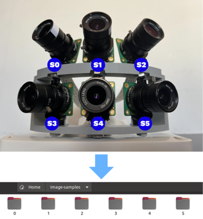
The content of each folder will be samples of images of the specific camera index. The images must use the name format image_sXX_YY with XX being the camera index and YY the sample index.
The images of each sensor should be in sync (all captured at the same time) to achieve the images overlap. |
An example of the hierarchical structure of the root folder for an array of three cameras looks like this:
root_folder
├── 0
│   ├── image_s0_00.jpeg
│   ├── image_s0_01.jpeg
│   ├── image_s0_02.jpeg
│   ├── image_s0_03.jpeg
│   ├── image_s0_04.jpeg
│   └── image_s0_05.jpeg
├── 1
│   ├── image_s1_00.jpeg
│   ├── image_s1_01.jpeg
│   ├── image_s1_02.jpeg
│   ├── image_s1_03.jpeg
│   └── image_s1_05.jpeg
└── 2
    ├── image_s2_00.jpeg
    ├── image_s2_01.jpeg
    ├── image_s2_02.jpeg
    ├── image_s2_03.jpeg
    ├── image_s2_04.jpeg
    └── image_s2_05.jpeg
Image Details
To calculate the homography matrices, the calibration tool first calculates and matches the features of a pair of images in the overlap section. To perform a good and easier calibration the sample images much follow the following characteristics:
- Capture images with good light conditions.
- Capture distinctive objects in the overlapping sections of the camera setup.
Camera order assignment
The calibration tool arranges the images in the order of the input folders from 0 to N-1 cameras, with images in folder 0 as reference and images from folders 1 to N-1 as target. To go through all the cameras use the next button.
The tool uses the images in the order of folders 0, 1, 2... N-1 with folder 0 as reference. In case the camera index 0 does not correspond to the reference, save the respective camera samples in folder 0. For example, if the reference camera has the index 4 save the image samples from camera 4 in folder 0.

We recommend using as reference the center images. For example, in the configuration above we use as a reference the camera index 4 followed by its adjacent images, the hierarchical structure of the folder looks like:
cameras-sampĺes
├── 0
│   ├── image_s4_00.jpeg
│   ├── image_s4_01.jpeg
│   ├── image_s4_02.jpeg
│   └── image_s4_03.jpeg
├── 1
│   ├── image_s3_00.jpeg
│   ├── image_s3_01.jpeg
│   ├── image_s3_02.jpeg
│   └── image_s3_03.jpeg
├── 2
│   ├── image_s5_00.jpeg
│   ├── image_s5_01.jpeg
│   ├── image_s5_02.jpeg
│   └── image_s5_03.jpeg
├── 3
│   ├── image_s1_00.jpeg
│   ├── image_s1_01.jpeg
│   ├── image_s1_02.jpeg
│   └── image_s1_03.jpeg
├── 4
│   ├── image_s0_00.jpeg
│   ├── image_s0_01.jpeg
│   ├── image_s0_02.jpeg
│   └── image_s0_03.jpeg
└── 5
    ├── image_s2_00.jpeg
    ├── image_s2_01.jpeg
    ├── image_s2_02.jpeg
    └── image_s2_03.jpeg
It is important that images for each folder overlap with the images of previous folders. For example, images in folder 3 must overlap with at least one of the images in folders 0, 1, or 2.
Sample images extraction
The sample images can be extracted from a video using ffmpeg or GStreamer. Follow the next steps to obtain the images directory using videos of each sensor of the setup.
If the video presents image distortion consider using the cuda-undistort element to record the videos or to convert the video files. |
- 1. Obtain videos of each sensor in the homography setup. For an easier calibration make sure to have different scenes with distinctive objects in the middle of the cameras overlap.
- 2. Create a root folder in the desired path to save the sensors samples folder. Inside the root folder create a folder for each sensor with the camera indexes starting from 0.
The root folder must contain only the numbered folders. For example for a setup of three cameras:
mkdir root_folder
cd root_folder
mkdir 0 1 2
- 3. Extract samples for each camera using ffmpeg or GStreamer.
The amount of extracted samples corresponds approximately to framerate (frames/second) * total_video_seconds. For example, you can set the framerate to capture a frame every 30 seconds using 1/30 as the framerate.
For ffmpeg use the following command:
ffmpeg -i <video_path> -r <framerate> <folder_path>/image_s<index>_%02d.jpg
For GStreamer in the case of videos encoded in h265 use the following command:
gst-launch-1.0 filesrc location=<video_path> ! qtdemux ! h265parse ! decodebin ! jpegenc ! multifilesink location= <folder_path>/image_s<sindex>_%02d.jpeg -v
Use these commands for each of the available sensors.
Calibration tool usage
- 1. To use the calibration tool run the following command and select the Panoramic Calibration button.
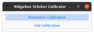
stitching-calibrator
- 2. Upload the sample images. In the menu bar select File->Load Images, this will open a file dialog to select the root directory with the cameras folders.
Note: To open the correct folder, search the directory of the folder and select the images root directory, once selected click Load Images.
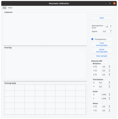

- 3. In the Overlap view, move the images to match the areas of overlap. Select the values of reprojection error and sigma.
- Reprojection error: Reprojection error for points inlier calculation. This parameter has a range of 1 to 10.
- Sigma: Sigma value for the Gaussian filter.
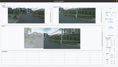
- 4. Proceed to calculate the homography using the Find Homography button. The homography will be displayed in the Homography view.
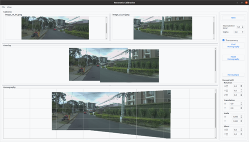
- 5. Automatic homography calculation can need adjusting. Use the following methods to adjust the resulting homography.
- Homography manual edition: Tune the current calculated homography using the transformations of the manual edit buttons.
The available transformations are:
- Rotation: Rotates the target image in x, y or z angle.
- Translation: Translate the target image in x or y axis.
- Scale: Scale the target image in x or y axis.
- Shear: Shear the target in x or y axis.

The transparency checkbox enable/disable transparency on the Homography view images, this feature facilitates the homography tuning. |
- Multiple samples calculation: Use the New Sample button to use the following samples for each of the cameras. Proceed to calculate a new homography with the Find Homography button. This new homography will use the matching features of past and current samples.
- 6. Once the current images homography is ready, press the button Next to continue with the following sensor and calculate the homography for the next target sensor. Continue until you estimate homographies for all sensors.
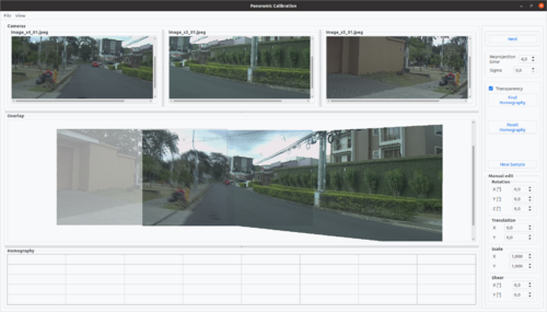
- 7. When the calibration is finished, save the homographies in a JSON file. In the menu bar select File->Export Calibration, this will open a file dialog to select the path and name for the JSON file.
An example of the JSON file output using three sensors looks like:
{
    "homographies": [
        {
            "images": {
                "target": 1,
                "reference": 0
            },
            "matrix": {
                "h00": 1.1946803311080263,
                "h01": -0.07181214798681632,
                "h02": 974.6987116573841,
                "h10": 0.05741935598536246,
                "h11": 0.9766926330946756,
                "h12": 28.023243439318392,
                "h20": 0.00011390078636798156,
                "h21": -8.400798382098214e-05,
                "h22": 1.0
            }
        },
        {
            "images": {
                "target": 2,
                "reference": 0
            },
            "matrix": {
                "h00": 1.0620898955373828,
                "h01": 0.00987091535047472,
                "h02": 996.497965020474,
                "h10": 0.03135702679953584,
                "h11": 1.0382444661991115,
                "h12": 7.544777297565004,
                "h20": 4.8771808894142367e-05,
                "h21": 9.65031537781453e-06,
                "h22": 1.0
            }
        }
    ]
    "state": [
        {
            "parameters": {
                "rotation_x": 20.0,
                "rotation_y": 0.0,
                "rotation_z": 0.0,
                "translation_x": 5.0,
                "translation_y": 0.0,
                "scale_x": 1.0,
                "scale_y": 1.0,
                "shear_x": 0.0,
                "shear_y": 0.0,
                "reproj_error": 4.0,
                "sigma": 0.0,
                "transparency": true
            },
            "homography": [
                [
                    1.000058762912872,
                    7.888498385152689e-05,
                    3199.4499814905034
                ],
                [
                    4.723958595481137e-05,
                    1.0000931533982886,
                    -0.08369247595611147
                ],
                [
                    2.5577758990969628e-08,
                    2.3474284624048636e-08,
                    1.0
                ]
            ]
        },
        {
            "parameters": {
                "rotation_x": 0.0,
                "rotation_y": 10.0,
                "rotation_z": 0.0,
                "translation_x": 0.0,
                "translation_y": 0.0,
                "scale_x": 1.0,
                "scale_y": 1.0,
                "shear_x": 0.0,
                "shear_y": 0.0,
                "reproj_error": 4.0,
                "sigma": 0.0,
                "transparency": true
            },
            "homography": [
                [
                    0.99999609783887,
                    -9.718761972552558e-06,
                    4925.1607901084235
                ],
                [
                    2.6465994305042002e-06,
                    0.9999954907576784,
                    0.0016865949159274893
                ],
                [
                    1.3692964877812703e-09,
                    -1.848738437444207e-09,
                    1.0
                ]
            ]
        }
    ]
}
The Calibration Tool also includes options to load a previously obtained calibration file or a project, which includes a calibration file and sample images. To load a calibration file upload the images as shown in step 2, and then load the calibration using the file menu, File->Load Calibration. A file dialog will appear so that you can select the desired JSON file. After the file is selected, the corresponding parameters saved in the file will be applied.

If you want to save a project, after loading images click File->Save Project, a file dialog will open so that you can select the location and name of your project. This project will be saved as a TAR file with the .stp extension.

To load a project, simply click File->Load Project in the menu. A file dialog will be opened to select the .stp project that you want to load. After the project is selected images contained in the project will be loaded and parameters saved in the calibration file inside the project will be applied.

The Homography Estimation tool has a dark mode feature. You can enable the dark theme in the menu View->Dark Mode.

We recommend you watch the following video in which we present you with a comprehensive tutorial on how to use the Stitching Calibrator for panoramic stitching.


