360 Calibration
| RidgeRun Image Projector |
|---|

|
| Image Projector Basics |
| Overview |
| Getting Started |
| User Guide |
| Examples |
| Performance |
|
Xavier
|
| Contact Us |
360 Calibration Tool
The following section will introduce how to calibrate the equirectangular projection that can be used in the rreqrprojector element. This tool consists of a Python application that estimates the equirectangular projection of fisheye images and the horizontal offset to match the images.
If you are not familiar with the tool, we recommend you to watch the following video :
Dependencies
- Python 3.8
- OpenCV headless
- Numpy
- PyQt5
- PyQtDarkTheme
Tool installation
It is recommended to work in a virtual environment since the required dependencies will be automatically installed. To create a new Python virtual environment, run the following commands:
ENV_NAME=calibration-env
python3 -m venv $ENV_NAME
A new folder will be created with the name ENV_NAME. To activate the virtual environment, run the following command:
source $ENV_NAME/bin/activate
In the directory of the stitching-calibrator project provided when you purchase the product, run the following command:
pip3 install --upgrade pip
pip3 install .
Tool Setup
In order to correctly upload the fisheye images to the calibration tool, a root folder with only a series of folders named with the camera indexes starting from 0, 1, 2, ... all the way up to the number of cameras of the array being calibrated. The content of each folder will be one fisheye image of the specific camera index. The fisheye images must use the name format image_XX with XX being the camera index.
The images of each sensor should be in sync (all captured at the same time) to achieve the images overlap. |
An example of the hierarchical structure of the root folder for an array of three fisheye cameras looks like this:
fisheye-images/
├── 0
│   └── image_0.jpeg
├── 1
│   └── image_1.jpeg
└── 2
    └── image_2.jpeg
Calibration tool usage
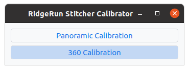
- 1. To use the calibration tool run the following command and select the 360 Calibration button.
stitching-calibrator
- 2. Upload the fisheye images. In the menu bar select File->Load Images, this will open a file dialog to select the root directory with the cameras folders.
Note: To open the correct folder, search the directory of the folder and select the images root directory, once selected click Open. |

An initial circle estimation and equirectangular projection will be estimated for each image, this will take a few seconds. The image of sensor 0 will be automatically selected in the Samples view to calibrate and highlight in the Cameras view.
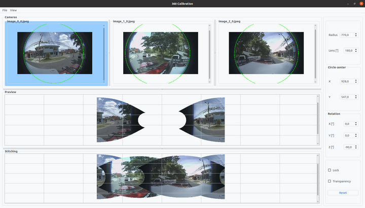
- 3. Adjust the parameter of the first fisheye image using the buttons of the right panel where:
- radius: A float property that defines in pixels the radius of the circle containing the fisheye image.
- lens: A float property that defines the fisheye lens aperture.
- circle-center-x: An integer property that defines the center position of the fisheye circle over the input’s image X axis(horizontal).
- circle-center-y: An integer property that defines the center position of the fisheye circle over the input’s image Y axis(vertical).
- rot-x: A float property that defines the camera’s tilt angle correction in degrees between -180 and 180. This is assuming a coordinate system over the camera where the X axis looks over the side of the camera, if you rotate that axis, you will be rotating the camera up and down.
- rot-y: A float property that defines the camera’s roll angle correction in degrees between -180 and 180. This is assuming a coordinate system over the camera where the camera lens looks over the Y axis, if you rotate that axis, the camera will rotate rolling over its center.
- rot-z: A float property that defines the camera’s pan angle correction in degrees between -180 and 180. This is assuming a coordinate system over the camera where the Z axis is over the camera, if you rotate that axis, the camera will pan over its center moving around the 360 horizon.
The Preview view will show the result projection of the selected image with the selected parameters.
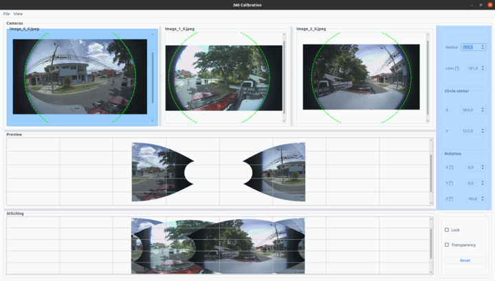
The view size can be individually adjusted using the slider for a better appreciation of the images, use scroll for vertical adjustment, and Shift+scroll for horizontal adjustment. Also, the images can be zoom in and zoom out using Ctrl+scroll. |
- 4. Select another sensor image in the Samples view (by clicking on it) to adjust the projection parameters for the next image, and continue with all the available sensor images. The current sensor image will be highlighted to recognize which image you are currently adjusting.
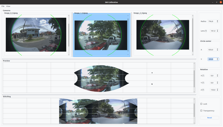
- 5. In the Stitching view the images are displayed one on top of the other one, this display allows the user to have a preview of the stitching result. If needed modify the parameters for each sensor to fit the features in the overlap area.
If the horizontal plane of the images doesn't match tune the Z Rotation parameter or drag the images in the Stitching view one on top of the other one and match the scene. Dragging the images will change the homography matrix from an identity to a translation matrix.
Note: Use the transparency and lock features to help you match the scene. |
The transparency feature allows transparent images to match objects between the projections. The lock feature locks the image movement for an easier projection tune.
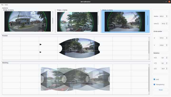
- 6. When the calibration is finished, save the parameters and homographies in a JSON file. In the menu bar select File->Export Calibration, this will open a file dialog to select the path and name for the JSON file.

An example of the JSON file output using two fisheye images looks like:
{
    "projections": [
        {
            "0": {
                "radius": 640.0,
                "lens": 195.0,
                "center_x": 637.0,
                "center_y": 640.0,
                "rot_x": 0.0,
                "rot_y": 0,
                "rot_z": 180,
                "fisheye": true
            }
        },
        {
            "1": {
                "radius": 639.0,
                "lens": 195.0,
                "center_x": 641.0,
                "center_y": 638.0,
                "rot_x": 0.0,
                "rot_y": -0.8,
                "rot_z": 180,
                "fisheye": true
            }
        }
    ],
    "homographies": [
        {
            "images": {
                "target": 1,
                "reference": 0
            },
            "matrix": {
                "h00": 1,
                "h01": 0,
                "h02": 1309.612371682265,
                "h10": 0,
                "h11": 1,
                "h12": 0,
                "h20": 0,
                "h21": 0,
                "h22": 1
            }
        }
    ]
}
The Calibration Tool also includes options to load a previously obtained calibration file or a project, which includes a calibration file and sample images. To load a calibration file upload the images as shown in step 2, and then load the calibration using the file menu, File->Load Calibration. A file dialog will appear so that you can select the desired JSON file. After the file is selected, the corresponding parameters saved in the file will be applied.

If you want to save a project, after loading images click File->Save Project, a file dialog will open so that you can select the location and name of your project. This project will be saved as a TAR file with the .st3 extension.

To load a project, simply click File->Load Project in the menu. A file dialog will be opened to select the .st3 project that you want to load. After the project is selected images contained in the project will be loaded and parameters saved in the calibration file inside the project will be applied.

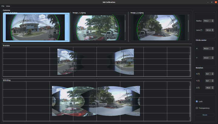
The Panoramic Calibration tool has a dark mode feature. You can enable the dark theme in the menu View->Dark Mode.
Projector usage example
The following examples show how to use the calibrator tool JSON output with the stitcher and the projector. This example uses the above JSON output example of two fisheye images as result.json.
Write the projection parameters of each sensor image from the JSON file to environment variables:
S0_C_X=637
S0_C_Y=640
S0_rad=640
S0_R_X=0
S0_R_Y=0
S0_LENS=195

S1_C_X=641
S1_C_Y=638
S1_rad=639
S1_R_X=0
S1_R_Y=-0.8
S1_LENS=195
The homography list can be used in the pipeline with the following format:
CONFIG_FILE="result.json"
HOMOGRAPHIES="`cat $CONFIG_FILE | tr -d "\n" | tr -d " "`"
Assuming the Calibrator tool output is stored in a result.json file, a full pipeline looks like:
S0_C_X=637
S0_C_Y=640
S0_rad=640
S0_R_X=0
S0_R_Y=0
S0_LENS=195

S1_C_X=641
S1_C_Y=638
S1_rad=639
S1_R_X=0
S1_R_Y=-0.8
S1_LENS=195

CONFIG_FILE="result.json"
HOMOGRAPHIES="`cat $CONFIG_FILE | tr -d "\n" | tr -d " "`"

GST_DEBUG=WARNING gst-launch-1.0 -e -v \
	cudastitcher name=stitcher homography-list=$HOMOGRAPHIES sink_0::right=1200 sink_1::right=1227 \
	filesrc location= ~/videos/video0-s0.mp4 ! qtdemux ! queue ! h264parse ! nvv4l2decoder ! queue ! nvvidconv ! rreqrprojector center_x=$S0_C_X center_y=$S0_C_Y radius=$S0_rad rot-x=$S0_R_X rot-y=$S0_R_Y lens=$S0_LENS name=proj0 !  queue ! stitcher.sink_0 \
	filesrc location= ~/videos/video0-s1.mp4 ! qtdemux ! queue ! h264parse ! nvv4l2decoder ! queue ! nvvidconv ! rreqrprojector center_x=$S1_C_X center_y=$S1_C_Y radius=$S1_rad rot-x=$S1_R_X rot-y=$S1_R_Y lens=$S1_LENS name=proj1 !  queue ! stitcher.sink_1 \
	stitcher.  ! queue ! nvvidconv ! nvv4l2h264enc bitrate=30000000 ! h264parse ! queue !  qtmux ! filesink location=360_stitched_video.mp4
We recommend you watch the following video in which we present you with a comprehensive tutorial on how to use the Stitching Calibrator for video 360 stitching.

