
Assembly Line Activity Recognition
Project summary
This project involves a complete machine learning activity recognition process: data capturing, labeling, developing the tools and training base, and finally parameter tuning and experimenting.
The final trained model is capable of detecting activities from an assembly line video at 45 frames per second, with accuracy, precision, recall, and f1-score above 0.913 using transfer learning. The project was built around PyTorchVideo's SlowFast implementation; our custom software allows us to experiment with this network for our specific use case, modify parameters and test multiple training and tuning techniques in order to achieve the best results possible.
The following video shows the inference results (in blue) as well as a manually labeled base (ground truth in green) for a test sample (these samples were not used for training).
Project context
As part of RidgeRun's intention to expand its solutions portfolio, the company is venturing into the field of machine learning with a special focus on deep learning applications for the industry such as activity recognition.
Industrial processes are great candidates for activity recognition based on machine learning and computer vision because it occurs in controlled environments, and the number of variables can be controlled and managed according to the task. So, RidgeRun partnered with a manufacturing company in the field of multimedia hardware to explore ways of automating the assembly validation process i.e. being able to automatically classify assembly actions so a further validation process can take place.
In order to provide automated assembly validation solutions, RidgeRun is testing and researching multiple smart activity recognition techniques. This project explores the viability of the deep learning approach and also provides the tools and workflow required for future similar applications.
The manufacturing third party provides the environment for data capture and the problem to be solved while RidgeRun provides all the development resources to tackle the problem, ranging from data capture to network training.
This project's tools, methodology, and knowledge can be applied to many other industrial environments and problems in order to automate, validate, monitor, and improve manufacturing processes. The improvements in products and their manufacturing complexity call for new and more advanced validation techniques, these new requirements are the driving force behind this project's development.
Problem description
Currently, the manufacturing company doesn't have an automatic way to recognize the actions performed on the assembly line, which can produce defective assembled parts that affect the quality of the final product.
The problem mentioned above can be addressed manually by monitoring the production line; however, this will result in inefficient use of resources and relies on human detection and decision making, which could be biased and inaccurate. The implementation of an automatic recognition system allows efficient validation of the assembly process without human intervention.
This project focuses on how to detect and recognize activities on an assembly line from video samples using machine learning and computer vision techniques.
Parts and workstation
The activities to be recognized are from an assembly line that utilizes six parts that are placed in a specific sequence by a worker in an assembly workstation. These parts are listed below:
- Riveted star
- Separator
- Spacer
- Washer
- Greased disk
- Lid
The assembly occurs at a static workstation where the parts are laid out in a particular order, making this problem a classification task instead of a detection task. The following figure shows the workstation where the parts are assembled and details how the parts are laid out. It also shows a number for each section of interest according to the following numbering:
- Riveted star
- Hand press
- Lid
- Greased disk
- Complete part
- Washer
- Separator
- Spacer

Activities definition
The labels are specified based on the assembly parts, these labels are also the activities that the network needs to learn to recognize. The following table shows these activities along with a brief description.
| ID | Label | Description |
|---|---|---|
| 0 | Install riveted star | The worker reaches and grabs a riveted star from its container/holder; then installs it on the assembly holder (under the hand press). |
| 1 | Install separator | The worker reaches and grabs a separator from its container/holder; then installs it on the assembly holder (under the hand press). |
| 2 | Install spacer | The worker reaches and grabs a spacer from its container/holder; then installs it on the assembly holder (under the hand press). |
| 3 | Install greased disk | The worker reaches and grabs a greased disk from its container/holder; then installs it on the assembly holder (under the hand press). |
| 4 | Install washer | The worker reaches and grabs a washer from its container/holder; then installs it on the assembly holder (under the hand press). |
| 5 | Install lid | The worker reaches and grabs a lid from its container/holder; then installs it on the assembly holder (under the hand press). |
| 6 | Press down | The worker grabs the white compression body, places it on top of the assembly holder, then pulls the handle and compresses the assembly body. |
| 7 | Complete part | The worker grabs the completed part from under the press and moves it to the side with all the completed parts. |
| 8 | Part removal | The worker removes an already placed part from the assembly holder (under the hand press) and puts it back in its container. |
Implementation details
This project development contemplates everything from data capturing all the way to network training and optimization. All of these stages are crucial to the final results. This section presents the process of data acquisition, data characterization and exploratory analysis, network code base implementation and finally the network configuration and training.
Dataset acquisition
This dataset was generated for activity recognition in production environments using supervised machine learning; therefore, it consists of video samples and their respective labels. However, it can be used for other video related activities or even image detection with little extra processing. As seen in the following table this dataset consists of 202 videos making up 36376 seconds of video, equivalent to around ten hours of playback.
| Field | Value |
|---|---|
| Number of observations (Annotations) | 42260 |
| Number of unique observations | 28128 |
| Number of variables | 8 |
| Number of used variables | 3 |
| Missing/corrupted samples | 0 |
| Labeled/trimmed videos | 202 |
| Duration of labeled videos | 36375.98467(s) |
| Size of labeled videos | 18746042815(bytes) |
These videos do not have a standard length, they were trimmed to avoid unwanted samples and dead times.
The video samples were extracted during the last quarter of 2021 using a prototype camera assembled at RidgeRun with the following specifications:
- SoC: NVIDIA Jetson Nano
- Sensor: Sony IMX477
- Storage: 1TB NVMe
- OS: Ubuntu 18.04 LTS
The software was developed by RidgeRun with the following specifications:
- Gstreamer-based solution.
- Camera acquisition and recording.
- Configurable recording schedule.
- Automatic recording splitting.
- WiFi access point connectivity.
- Wifi video preview.
The hardware was mounted diagonally from the workstation in a fixed position to ensure that all samples have the same point of view. The following image shows the camera installation for recording the videos used as input for this project.

Dataset characteristics
Each dataset sample is associated with a group of frames called a window, this window is 30 frames long (1 second). Each sample has a label associated with 2 additional fields besides the actual label: video-id and timestamp, in order to know what part of the video it is related to.
The labels are stored in a comma-separated file with the following structure:
video-id, timestamp, class
This represents a sample from a video called video-id with the window centered at timestamp (meaning from second timestamp - 0.5 to second timestamp + 0.5) and the activity is labeled as class.
A real sample looks like the following:
24-11-2021_06_00_17_01_(7).mp4,695.5,3
24-11-2021_06_00_17_01_(7).mp4,696.5,5
24-11-2021_06_00_17_01_(7).mp4,701.5,6
24-11-2021_06_00_17_01_(7).mp4,704.5,7
Exploratory Data Analysis (EDA)
Data is a key aspect of a successful machine learning application, a dataset must meet the correct characteristics in order to be used to train a neural network that produces good results. For the purpose of determining those characteristics in the assembly dataset, an Exploratory Data Analysis (EDA) was performed. The EDA allowed us to have a better understanding of the dataset composition, its weaknesses, and strengths, as well as foresee possible issues or biases during the training phase. The following plot shows the dataset class distribution.

From this EDA it was concluded that the Part Removal label was too represented, only 0.35% of the labels fell under this category which makes it really complicated to train a network for this case. Based on this and other experimental results it was decided that this class was not going to be used for the final network training.
The EDA also included a visualization process for the class samples, this helped determine any dependency between classes. As a result, it was noted that the Install spacer and Install washer labels happened together in most of the video samples, which means that there were no unique samples for training; this resulted in the combination of these classes into a new one called Install spacer and washer.
Network implementation
The project uses a SlowFast architecture, which is a 3D convolutional neural network with two main data paths, it uses a slow and a fast path, these paths specialize either in spatial data or in temporal data, to make a complete spatiotemporal data processing.
The network used is a PyTorch implementation from the PyTorchVideo library. The following figure shows a basic representation of the layers that constitute this network.

This project was built around this PyTorchVideo SlowFast implementation; the software allows us to experiment with this network for our specific use case, modify parameters and test multiple training and tuning techniques in order to achieve the best results possible. For experiment tracking and reproducibility this project was built using DVC as an MLOps tool, with a 5-stage process as seen in the following dependency diagram.

Network configuration
The process to find the parameters that yield the best performance in a network for a particular problem is one of the most complex parts of machine learning applications. Some of the experiments that were tested for this project are described below, this process was performed incrementally, improving the network over time.
- Transfer learning.
- Data subsampling.
- Data replacement.
- Weighted cross-entropy.
- Focal loss.
- Complete dataset training.
- Remove underrepresented classes.
- Cross-validation.
Transfer learning
For the experimentation process, baseline training was executed in order to have a point of reference and a starting point. After the baseline was executed, the first decision to make was whether to use transfer learning or keep the training process from scratch. The results from using transfer learning yielded the biggest improvement in the network performance; we used a SlowFast model from torch hub that was trained on the kinetics 400 datasets. This achieved twice as better performance in one-fourth of the time compared to training from scratch. Transfer learning improved the training times as well as the network performance. The following plots show the difference between transfer learning and the baseline confusion matrices.
-
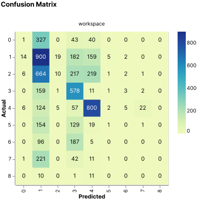 Baseline confusion matrix
 -
 Transfer learning confusion matrix


Classes subsampling and replacement
The next problem that needed solving was the data imbalance present in the dataset. As seen in the original data distribution plot, the dataset was not balanced and some classes were underrepresented. To tackle this problem, the first technique tested was the dataset subsampling, where not all samples available were used; only selected samples from each class were in order to keep a balanced distribution. This was not optimal since a lot of useful data was being left out; after that, data replication was introduced where samples were selected with replacement. This was also not ideal since samples for the underrepresented classes were repeated a lot in the dataset. Finally, different loss functions were tested, particularly weighted cross entropy and focal loss, both of which account for the data distribution to calculate the loss. This is what yielded the best results and led to the use of focal loss for all experiments going forward. The following plots show the original baseline dataset distribution and the final distribution used for most of the experiments; this also includes the removal of underrepresented labels.
-
 Baseline dataset
 -
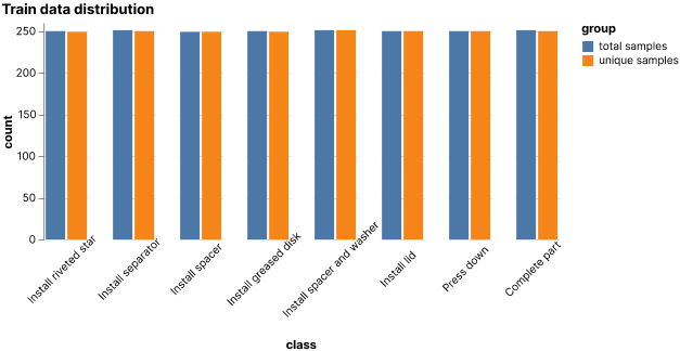 Dataset distribution after class balancing


Overfitting
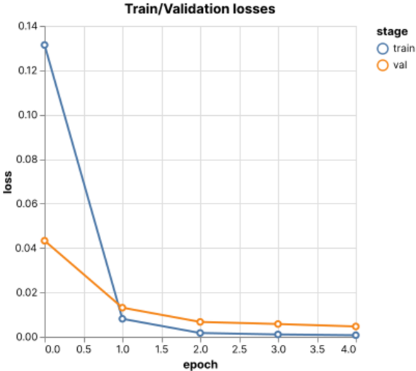
Once the data imbalance problem was tackled, the next problem was overfitting, this can be seen in the image below extracted from the balanced training using transfer learning, where the validation loss plot crosses the training loss plot indicating that the validation loss does not decrease at the same rate as the training loss and therefore the network is overfitting to the training dataset.
To solve this the first experiment was training with more data, specifically with the complete dataset; this however, did not reduce the overfit, so the next experiment was to remove the underrepresented classes such as Part Removal, this had an improvement over the network but the overfit remained; finally the training approach was changed to use cross-validation which solved the overfitting issue and it was kept for the final training. The following image shows the result of cross-validation training and how both plots do not cross anymore.
-
 Loss plots overfitting behaviour
 -
 Cross validation training (no overfit)


Final configuration
From the experimentation process the best configuration and parameters were extracted for the final model which was also the one with the best performance; it was trained using transfer learning from a Kinetics 400 SlowFast model from PyTorchVideo's model hub; this model was trained using focal loss and cross-validation to avoid overfitting.
The training was performed over 5 epochs in batches of 8 using 5 cross validation folds. In addition, the Stochastic Gradient Descent optimizer was used with a learning rate of 0.001 and 0.9 momentum. The model results are presented in the next section.
Results
The network was tested on a separate part of the dataset, that had not been presented to the network. The best-performing model achieved an accuracy of 0.91832, a precision of 0.91333, a recall value of 0.91832, and finally an f1-score of 0.91521. These metrics indicate a very high performance of the network for this particular task; the following table presents the complete training, validation, and testing results.
| Metric | Value |
|---|---|
| train_accuracy | 0.99932 |
| train_precision | 0.99936 |
| train_recall | 0.99932 |
| train_f1_score | 0.99934 |
| train_loss | 0.00070697 |
| val_accuracy | 0.99577 |
| val_precision | 0.99478 |
| val_recall | 0.99577 |
| val_f1_score | 0.99526 |
| val_loss | 0.0046519 |
| test_accuracy | 0.91832 |
| test_precision | 0.91333 |
| test_recall | 0.91832 |
| test_f1_score | 0.91521 |
In addition, the following plots show the training and validation loss for the best-performing network, as well as the test confusion matrix; this matrix shows predominance along its diagonal; indicating a match between the networks predictions and the sample's ground truth.
-
 Loss plots
 -
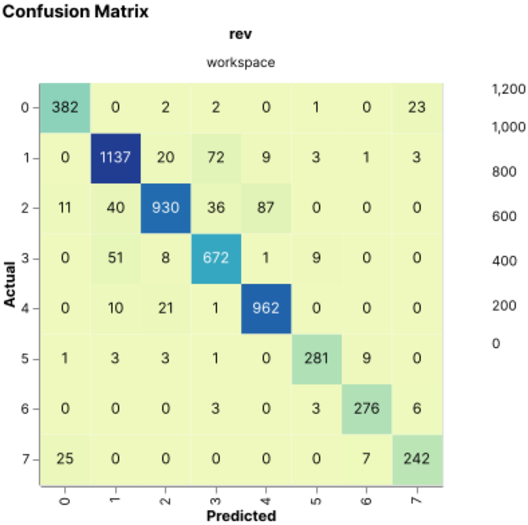 Confusion matrix (5354 samples)


Finally, the inference demo below shows a gif of the assembly process under inference; it displays the top prediction for the sample as well as the associated softmax value. This inference process has a threshold of 0.5 meaning that if none of the softmax values achieve a 50% value, then no activity is recognized.

Inference performance
In terms of performance; the complete process as it is takes 1.115 seconds on average to perform inference over a sample; however, this considers the process of loading and trimming the sample as well as normalizing and transforming it for the network. The inference itself, once the sample preprocessing is done, only takes 22.1ms for each sample. These measurements were performed on a Google Cloud Platform VM, with the following hardware specifications:
- CPU: Intel(R) Xeon(R) CPU @ 2.30GHz
- MEM: 32GB Ram
- GPU: NVIDIA Tesla T4
The sample preprocessing could be accelerated since it is currently not running on the GPU; however, by excluding this time, we can assure that the network is capable of performing inference at around 45 frames per second, but is currently limited at 0.91 frames per second due to inefficient preprocessing. The following table shows the results of the inference performance measurements over 50 samples.
| Measurement | Value |
|---|---|
| Samples | 50 |
| Aggregated processing and inference time (s) | 55.7563 |
| Average processing and inference time (s) | 1.1151 |
| Aggregated inference only time (s) | 1.1056 |
| Average inference only time (s) | 0.02211 |
What is next?
Having a trained model for the specific assembly process allows getting a prediction in real time of every action that happens during production. These predictions can be used for online analysis of the production process into an embedded system, and automatically flag the recorded videos when a specific set of events happen such as a part is removed, the assembly sequence is incorrect or a part has been completed. All this data can be automatically logged into the system and tied to the recorded video for posterior analysis. Remote configuration can be enabled on the edge device to allow the user to control the settings of the detection such as what events to log, change the recording settings, and change the behavior of specific events, among others. The following figure shows a simplified diagram of the entire solution for a production line:

Contact Us
For direct inquiries, please refer to the contact information available on our Contact page. Alternatively, you may complete and submit the form provided at the same link. We will respond to your request at our earliest opportunity.
Links to RidgeRun Resources and RidgeRun Artificial Intelligence Solutions can be found in the footer below.
ARTIFICIAL INTELLIGENCE