GstNetBalancer/Examples/Demo: Difference between revisions
m (Add demo images) |
m (Update image labels) |
||
| Line 3: | Line 3: | ||
</noinclude> | </noinclude> | ||
== Demo usecase == | |||
Suppose you have a 1280x720 video, encoded in H264 and running at 30fps. Also, consider the | In order to demonstrate the usage of the GstNetBalancer to optimize a network stream, consider the following case. | ||
Suppose you have a 1280x720 video, encoded in H264 and running at 30fps. Also, consider the stream uses MPEG-TS as the streaming protocol. The following sample pipeline can be used to replicate this scenario: | |||
<pre> | <pre> | ||
| Line 13: | Line 15: | ||
</pre> | </pre> | ||
If we take a look at the network usage graph, it looks like figure | If we take a look at the network usage graph, it looks like figure 1. Note that the peaks of the transmission graph reach about 600000 bits/ms which translates to about 600Mbps. This bandwidth requirement is notoriously wrong and beyond the capabilities of any common wireless network. Moreover, when reaching a limited network, packets are going to be dropped and the artifacts will become visible at the reception side. | ||
[[File:Gstnetbalancer unoptimized curve.png|center|frame|Figure | [[File:Gstnetbalancer unoptimized curve.png|center|frame|Figure 1. Bandwidth curve for an unoptimized pipeline. Video is 720p30 encoded in H264 and streamed using MPEG-TS]] | ||
If we take a closer look at the graph, it will look like figure | If we take a closer look at the graph, it will look like figure 2. Note that instead of sending the data packets distributed along the 33ms window (for a 30fps video), the packets are being sent as fast as possible, causing the transmission peak. | ||
[[File:Gstnetbalancer unoptimized pipeline zoomed.png|center|frame|Figure | [[File:Gstnetbalancer unoptimized pipeline zoomed.png|center|frame|Figure 2. Zoomed bandwidth curve for an unoptimized streaming pipeline. Note how all packets are sent as fast as possible instead of using all the frame rate window.]] | ||
In this demo, we are going to learn how to distribute the data packets along the frame rate window using GstNetBalancer. This will allow us to flatten the bandwidth curve and reduce the bandwidth requirements. | In this demo, we are going to learn how to distribute the data packets along the frame rate window using the GstNetBalancer. This will allow us to flatten the bandwidth curve and reduce the bandwidth requirements. | ||
The first step towards optimizing the example is to reduce the bandwidth required to some sort of acceptable value. First, remember that our video is an H264 720p@30 stream, so the video is compressed and each frame ends up with a different size. That said, it is not possible to calculate the exact required bandwidth based on the raw frame size but we can easily estimate it. We can use the following pipeline to look at the size of each encoded frame: | |||
The | |||
<pre> | <pre> | ||
| Line 30: | Line 31: | ||
</pre> | </pre> | ||
The previous pipeline will result in an output like the following: | |||
<pre> | <pre> | ||
| Line 40: | Line 41: | ||
</pre> | </pre> | ||
Looking at the last part of the log, it shows the value of one keyframe in the streaming (identified from its flags). For this specific keyframe, its size is 48494 bytes. Since we didn't use a more reliable way to estimate the size of the keyframes, we can just round up the sample and say we might be expecting keyframes around 50000 bytes - hoping most of the frames fall within this limit. Ideally more samples can be gathered and averaged. We will later see that this approximation leads us to close results and just some minimum tuning will be required to achieve the desired result. With all of this, let’s define the target bandwidth as: | |||
<pre> | <pre> | ||
| Line 46: | Line 47: | ||
</pre> | </pre> | ||
This way, we have already found the value for our first property bandwidth=12000 (remember it is defined on kbps units). | This way, we have already found the value for our first property '''bandwidth=12000''' (remember it is defined on kbps units). | ||
Our next property is the distribution-factor. In this case, we select it so that we ensure at least 10 transfer intervals within a frame window (33ms). Given we are running at 30fps we will need: | Our next property is the distribution-factor. In this case, we select it so that we ensure at least 10 transfer intervals within a frame window (33ms). Given we are running at 30fps we will need: | ||
| Line 55: | Line 56: | ||
There is not a specific rule behind our selection for the distribution-factor, we only want to make sure we have several opportunities to transfer packets within a frame interval. | There is not a specific rule behind our selection for the distribution-factor, we only want to make sure we have several opportunities to transfer packets within a frame interval. | ||
At this point, we can make a quick checkpoint and see what our bandwidth curve looks like. For this, we need to add the netbalancer element to our pipeline, just right before sending the packets to the network (since this is what we want to control). The following pipeline adds the netbalancer element with the settings calculated so far: | At this point, we can make a quick checkpoint and see what our bandwidth curve looks like. For this, we need to add the netbalancer element to our pipeline, just right before sending the packets to the network (since this is what we want to control). The following pipeline adds the netbalancer element with the settings calculated so far: | ||
| Line 63: | Line 63: | ||
</pre> | </pre> | ||
With this initial setup, we can get the bandwidth curves shown in figure | With this initial setup, we can get the bandwidth curves shown in figure 3. | ||
[[File:Gstnetbalancer partially optimized demo.png|center|frame|Figure | [[File:Gstnetbalancer partially optimized demo.png|center|frame|Figure 3. Bandwidth curve using netbalancer with bandwidth=12000 and distribution-factor=300]] | ||
Note that with just setting the proper bandwidth and distribution-factor, it has been possible to decrease the peak bandwidth from ~600Mbps to ~80Mbps, representing a reduction of 7.5 times. However, despite we have been able to decrease the required bandwidth for the video transmission, we are still running too high for normal wireless links (~20Mbps). If we look closer to the bandwidth curve (figure | Note that with just setting the proper bandwidth and distribution-factor, it has been possible to decrease the peak bandwidth from ~600Mbps to ~80Mbps, representing a reduction of 7.5 times. However, despite we have been able to decrease the required bandwidth for the video transmission, we are still running too high for normal wireless links (~20Mbps). If we look closer to the bandwidth curve (figure 4), we will notice that there is still some room between each data transfer to distribute more the packets. Our next step configuring the min-delay property will allow us to get closer to the estimated required bandwidth of 12Mpbs. | ||
[[File:Gstnetbalancer partially optimized demo zoomed.png|center|frame|Figure | [[File:Gstnetbalancer partially optimized demo zoomed.png|center|frame|Figure 4. Looking closer at the bandwidth curve, it is possible to note that there is still too much lost time within each transfer interval, and we can use this time to distribute the packets better.]] | ||
In order to select the proper min-delay for our case, we need to go a little bit deeper in the match and know the properties of our streaming configuration. First, since our target is 12Mpbs, we know this means a total transfer of 1.5MB/s. Considering a distribution-factor of 300 we can calculate the maximum amount of bytes to be transferred on each transfer interval: | In order to select the proper min-delay for our case, we need to go a little bit deeper in the match and know the properties of our streaming configuration. First, since our target is 12Mpbs, we know this means a total transfer of 1.5MB/s. Considering a distribution-factor of 300 we can calculate the maximum amount of bytes to be transferred on each transfer interval: | ||
<pre> | |||
bytes-per-interval = 1.5MB / 300 = 5000 bytes/interval | bytes-per-interval = 1.5MB / 300 = 5000 bytes/interval | ||
</pre> | |||
Additionally, we know that each transfer interval is performed on <code>3.3ms steps (1s / 300)</code> and considering <code>1MTU ~ 1400bytes</code> we can calculate the required min-delay as follows: | |||
<pre> | |||
# MTUs per interval = 5000 / 1400 = 3.57 MTUs | # MTUs per interval = 5000 / 1400 = 3.57 MTUs | ||
min-delay = 3.3ms / 3.57 = 924us | min-delay = 3.3ms / 3.57 = 924us | ||
</pre> | |||
Note that min-delay looks for distributing the packets to be sent over the network within the transfer interval, its value depends on the size of the data packets i.e. if we are using jumbo packets or 188-byte TS packets, then we need to do a new calculation. | Note that min-delay looks for distributing the packets to be sent over the network within the transfer interval, its value depends on the size of the data packets i.e. if we are using jumbo packets or 188-byte TS packets, then we need to do a new calculation. | ||
Anyway, at this point, we have a very good estimate of our min-delay, and we just need to tune it a little bit to compensate for our estimations. Rounding it up to 1000us as shown in the pipeline below, provides the curve shown in figure | Anyway, at this point, we have a very good estimate of our min-delay, and we just need to tune it a little bit to compensate for our estimations. Rounding it up to 1000us as shown in the pipeline below, provides the curve shown in figure 4. As it is possible to note, we have now reduced the required streaming bandwidth to about 15Mbps, which represents a reduction of about 40 times from our starting bandwidth (600Mbps). | ||
<pre> | <pre> | ||
| Line 92: | Line 92: | ||
</pre> | </pre> | ||
[[File:Gstnetbalancer optimized demo.png|center|frame|Figure | [[File:Gstnetbalancer optimized demo.png|center|frame|Figure 4. Optimized bandwidth curve using netbalancer.]] | ||
Finally, figure | Finally, figure 5 shows a zoomed version of the resulting bandwidth curve, note how the curve is almost flat with all packets distributed along the frame time. | ||
[[File:Gstnetbalancer optimized demo zoomed.png|center|frame|Figure | [[File:Gstnetbalancer optimized demo zoomed.png|center|frame|Figure 5. Looking closer at the optimized curve, it is possible to note that all packets have been distributed along the frame interval, making good use of the network bandwidth. | ||
]] | |||
This way, we have been able to demonstrate how GstNetBalancer can help to make correct use of your network bandwidth and optimize it at maximum, reducing the probability of packet loss and thus, reducing the artifacts when streaming video. | This way, we have been able to demonstrate how GstNetBalancer can help to make correct use of your network bandwidth and optimize it at maximum, reducing the probability of packet loss and thus, reducing the artifacts when streaming video. | ||
Revision as of 15:45, 14 October 2022
| GstNetBalancer A GStreamer Network Balancer Element |
|---|
 |
| About NetBalancer Plugin |
| Getting Started |
| User Guide |
| Examples |
| Contact Us |
Demo usecase
In order to demonstrate the usage of the GstNetBalancer to optimize a network stream, consider the following case.
Suppose you have a 1280x720 video, encoded in H264 and running at 30fps. Also, consider the stream uses MPEG-TS as the streaming protocol. The following sample pipeline can be used to replicate this scenario:
HOST_IP=192.168.1.10
PORT=3000
gst-launch-1.0 videotestsrc is-live=true ! 'video/x-raw,width=1280,height=720,framerate=30/1' ! queue ! x264enc key-int-max=30 bitrate=10000 ! queue ! mpegtsmux alignment=7 ! udpsink port=$PORT host=$HOST_IP -v
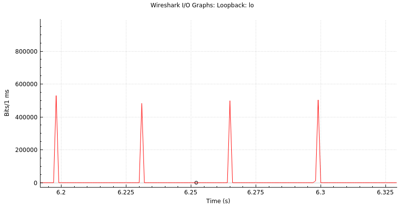
If we take a look at the network usage graph, it looks like figure 1. Note that the peaks of the transmission graph reach about 600000 bits/ms which translates to about 600Mbps. This bandwidth requirement is notoriously wrong and beyond the capabilities of any common wireless network. Moreover, when reaching a limited network, packets are going to be dropped and the artifacts will become visible at the reception side.

If we take a closer look at the graph, it will look like figure 2. Note that instead of sending the data packets distributed along the 33ms window (for a 30fps video), the packets are being sent as fast as possible, causing the transmission peak.
In this demo, we are going to learn how to distribute the data packets along the frame rate window using the GstNetBalancer. This will allow us to flatten the bandwidth curve and reduce the bandwidth requirements.
The first step towards optimizing the example is to reduce the bandwidth required to some sort of acceptable value. First, remember that our video is an H264 720p@30 stream, so the video is compressed and each frame ends up with a different size. That said, it is not possible to calculate the exact required bandwidth based on the raw frame size but we can easily estimate it. We can use the following pipeline to look at the size of each encoded frame:
gst-launch-1.0 videotestsrc is-live=true ! 'video/x-raw,width=1280,height=720,framerate=30/1' ! queue ! x264enc key-int-max=30 bitrate=10000 ! queue ! identity silent=false ! fakesink -v
The previous pipeline will result in an output like the following:
/GstPipeline:pipeline0/GstIdentity:identity0: last-message = chain   ******* (identity0:sink) (42170 bytes, dts: 1000:00:06.566666666, pts: 1000:00:06.633333333, duration: 0:00:00.033333333, offset: -1, offset_end: -1, flags: 00002000 delta-unit , meta: none) 0x7f1fe00597e0
/GstPipeline:pipeline0/GstIdentity:identity0: last-message = chain   ******* (identity0:sink) (42296 bytes, dts: 1000:00:06.600000000, pts: 1000:00:06.666666666, duration: 0:00:00.033333334, offset: -1, offset_end: -1, flags: 00002000 delta-unit , meta: none) 0x7f1fe003ad80
/GstPipeline:pipeline0/GstIdentity:identity0: last-message = chain   ******* (identity0:sink) (41148 bytes, dts: 1000:00:06.633333333, pts: 1000:00:06.700000000, duration: 0:00:00.033333333, offset: -1, offset_end: -1, flags: 00002000 delta-unit , meta: none) 0x7f1fe002c120
/GstPipeline:pipeline0/GstIdentity:identity0: last-message = chain   ******* (identity0:sink) (41121 bytes, dts: 1000:00:06.666666666, pts: 1000:00:06.733333333, duration: 0:00:00.033333333, offset: -1, offset_end: -1, flags: 00002000 delta-unit , meta: none) 0x7f1fe000ec60
/GstPipeline:pipeline0/GstIdentity:identity0: last-message = chain   ******* (identity0:sink) (48494 bytes, dts: 1000:00:06.700000000, pts: 1000:00:06.766666666, duration: 0:00:00.033333334, offset: -1, offset_end: -1, flags: 00000000 , meta: none) 0x7f1fe
Looking at the last part of the log, it shows the value of one keyframe in the streaming (identified from its flags). For this specific keyframe, its size is 48494 bytes. Since we didn't use a more reliable way to estimate the size of the keyframes, we can just round up the sample and say we might be expecting keyframes around 50000 bytes - hoping most of the frames fall within this limit. Ideally more samples can be gathered and averaged. We will later see that this approximation leads us to close results and just some minimum tuning will be required to achieve the desired result. With all of this, let’s define the target bandwidth as:
bandwidth = bytes-per-frame * bits-per-byte * frames-per-second = 50000 * 8 * 30 = 12Mpbs
This way, we have already found the value for our first property bandwidth=12000 (remember it is defined on kbps units).
Our next property is the distribution-factor. In this case, we select it so that we ensure at least 10 transfer intervals within a frame window (33ms). Given we are running at 30fps we will need:
distribution-factor = number-intervals-per-frame * frame-rate = 10 * 30 = 300
There is not a specific rule behind our selection for the distribution-factor, we only want to make sure we have several opportunities to transfer packets within a frame interval.
At this point, we can make a quick checkpoint and see what our bandwidth curve looks like. For this, we need to add the netbalancer element to our pipeline, just right before sending the packets to the network (since this is what we want to control). The following pipeline adds the netbalancer element with the settings calculated so far:
gst-launch-1.0 videotestsrc is-live=true ! 'video/x-raw,width=1280,height=720,framerate=30/1' ! queue ! x264enc key-int-max=30 bitrate=10000 ! queue ! mpegtsmux alignment=7 ! netbalancer bandwidth=12000 distribution-factor=300 ! udpsink port=3000 host=127.0.0.1 -v
With this initial setup, we can get the bandwidth curves shown in figure 3.
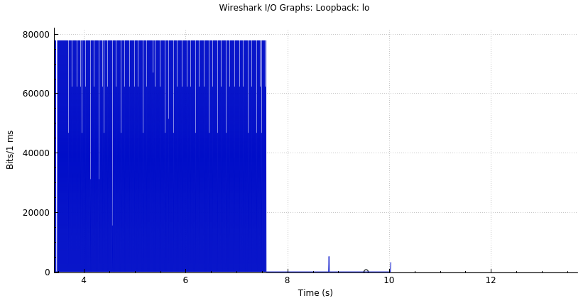
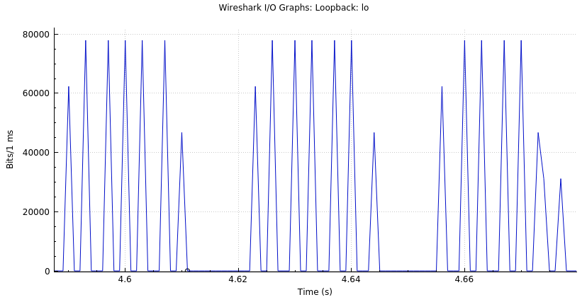
Note that with just setting the proper bandwidth and distribution-factor, it has been possible to decrease the peak bandwidth from ~600Mbps to ~80Mbps, representing a reduction of 7.5 times. However, despite we have been able to decrease the required bandwidth for the video transmission, we are still running too high for normal wireless links (~20Mbps). If we look closer to the bandwidth curve (figure 4), we will notice that there is still some room between each data transfer to distribute more the packets. Our next step configuring the min-delay property will allow us to get closer to the estimated required bandwidth of 12Mpbs.
In order to select the proper min-delay for our case, we need to go a little bit deeper in the match and know the properties of our streaming configuration. First, since our target is 12Mpbs, we know this means a total transfer of 1.5MB/s. Considering a distribution-factor of 300 we can calculate the maximum amount of bytes to be transferred on each transfer interval:
bytes-per-interval = 1.5MB / 300 = 5000 bytes/interval
Additionally, we know that each transfer interval is performed on 3.3ms steps (1s / 300) and considering 1MTU ~ 1400bytes we can calculate the required min-delay as follows:
# MTUs per interval = 5000 / 1400 = 3.57 MTUs
min-delay = 3.3ms / 3.57 = 924us
Note that min-delay looks for distributing the packets to be sent over the network within the transfer interval, its value depends on the size of the data packets i.e. if we are using jumbo packets or 188-byte TS packets, then we need to do a new calculation.
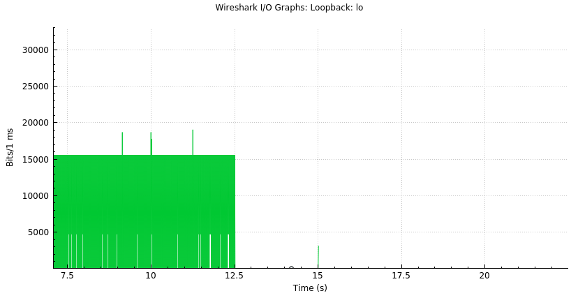
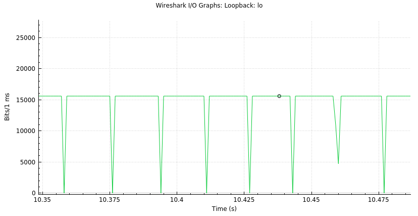
Anyway, at this point, we have a very good estimate of our min-delay, and we just need to tune it a little bit to compensate for our estimations. Rounding it up to 1000us as shown in the pipeline below, provides the curve shown in figure 4. As it is possible to note, we have now reduced the required streaming bandwidth to about 15Mbps, which represents a reduction of about 40 times from our starting bandwidth (600Mbps).
gst-launch-1.0 videotestsrc is-live=true ! 'video/x-raw,width=1280,height=720,framerate=30/1' ! queue ! x264enc key-int-max=30 bitrate=10000 ! queue ! mpegtsmux alignment=7 ! netbalancer bandwidth=12000 distribution-factor=300 min-delay=1000 ! udpsink port=3000 host=127.0.0.1 -v
Finally, figure 5 shows a zoomed version of the resulting bandwidth curve, note how the curve is almost flat with all packets distributed along the frame time.
This way, we have been able to demonstrate how GstNetBalancer can help to make correct use of your network bandwidth and optimize it at maximum, reducing the probability of packet loss and thus, reducing the artifacts when streaming video.
